Algorithms
An algorithm is step-by-step set of instructions for completing a task.
Searching
In computer science, a search algorithm is any algorithm which solves the search problem, namely, to retrieve information stored within some data structure, or calculates in the search space of a problem domain, either with discrete or continuous values.
For now, we are going to go over two different types of searches:
- Linear Search
- Binary Search
For the following examples, we are going to be using a row of lockers with numbers inside (an array) and we will look through them to find something, while returning a boolean (true or false) as a result.
A linear search is where we move in a line (usually start to end or end to start). The idea of the algorithm is to iterate across the array from left to right, searching for a specified element.
Worst-case scenario: We have to look through the entire array of n elements, either because the target element is the last element of the array or doesn't exist in the array at all.
Best-case scenario: The target element is the first element of the array, and so we can stop looking immediately after we start.
Now lets look through the lockers to find one with the number 50 inside. Some pseudocode for linear search could be written as:
For i from 0 to n–1  // from start (0) to end (n-1)
    If i'th element is 50
        Return true  // if the i'th element is 50 - return true
Return false // if not 50, return false
A binary search is where we start in the middle and move left or right, depending on what we're looking for. "Divide & Conquer". In order to leverage the power of binary search, our array must be sorted, else we cannot make assumptions about the array's content.
Worst-case scenario: We have to divide a list of n elements in half repeatedly to find the target element, either because the target element will be found at the end of the last division or doesn't exist in the array at all.
Best-case scenario: The target element is at the midpoint of the full array, and so we can stop looking immediately after we start.
Some pseudocode for binary search could be written as:
If no items
    Return false
If middle item is 50
    Return true
Else if 50 < middle item
    Search left half
Else if 50 > middle item
    Search right half
Big O
Computer scientists have created a way to describe algorithms (how well it is designed), and it's generally called big O.
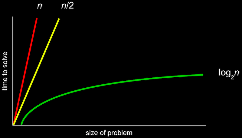
The more formal way to describe this is with big O notation, which we can think of as “on the order of”. For example, if our algorithm is linear search, it will take approximately O(n) steps, “on the order of n”. In fact, even an algorithm that looks at two items at a time and takes n/2 steps has O(n). This is because, as n gets bigger and bigger, only the largest term, n, matters.
There are some common running times (how many seconds does it take, how many steps does it take, etc.):
(lower is better)
- O(n2)
- O(n log n)
- O(n) (linear search)
- O(log n) (binary search)
- O(1)
Computer scientists might also use big Ω, big Omega notation, which is the lower bound of number of steps for our algorithm. (Big O is the upper bound of number of steps, or the worst case, and typically what we care about more.) With linear search, for example, the worst case is n steps, but the best case is 1 step since our item might happen to be the first item we check. The best case for binary search, too, is 1 since our item might be in the middle of the array.
And we have a similar set of the most common big Ω running times:
(lower is better)
- Ω(n2)
- Ω(n log n)
- Ω(n) (counting the number of items)
- Ω(log n)
- Ω(1) (linear search, binary search)
Linear Search
Now let's create a program to better visualize a lienar search:
1 2 3 4 5 6 7 8 9 10 11 12 13 14 15 16 17 18 | |
Here we initialize an array with some values, and we check the items in the array one at a time, in order.
And in each case, depending on whether the value was found or not, we can return an exit code of either 0 (for success) or 1 (for failure).
We can do the same for names:
1 2 3 4 5 6 7 8 9 10 11 12 13 14 15 16 17 18 19 | |
We can’t compare strings directly, since they’re not a simple data type but rather an array of many characters, and we need to compare them differently. Luckily, the string library has a strcmp function which compares strings for us and returns 0 if they’re the same, so we can use that.
Now lets implement a phone book with the same ideas:
1 2 3 4 5 6 7 8 9 10 11 12 13 14 15 16 17 18 19 | |
Now, if the name at a certain index in the names array matches who we’re looking for, we’ll return the phone number in the numbers array, at the same index. But that means we need to particularly careful to make sure that each number corresponds to the name at each index, especially if we add or remove names and numbers.
Let's improve the above code using our own custom data type!
Structs
We can make our own custom data types called structs:
1 2 3 4 5 6 7 8 9 10 11 12 13 14 15 16 17 18 19 20 21 22 23 24 25 26 27 28 29 30 31 32 33 34 35 36 37 38 39 | |
We can think of structs as containers, inside of which are multiple other data types.
Here, we create our own type with a struct called person, which will have a string called name and a string called number. Then, we can create an array of these struct types and initialize the values inside each of them, using a new syntax, ., to access the properties of each person.
In our loop, we can now be more certain that the number corresponds to the name since they are from the same person element.
Sorting
The process of Sorting can be explained as a technique of rearranging the elements in any particular order, which can be set ready for further processing by the program logic. In C, there are multiple sorting algorithms available, which can be incorporated inside the code.
Bubble Sort
In bubble stort, the idea of the algorithm is to move higher valued elements generally towards the right and lower value elements generally towards the left.
Let's take 8 random numbers (6, 3, 8, 5, 2, 7, 4, 1) and try to sort them in C.
First, we can look at the first two numbers and swap them so they are in order:
| 6 | 3 | 8 | 5 | 2 | 7 | 4 | 1 |
|---|---|---|---|---|---|---|---|
 |  | ||||||
| 3 | 6 | 8 | 5 | 2 | 7 | 4 | 1 |
The next pair, 6 and 8, are in order, so we don’t need to swap them.
The next pair, 8 and 5, need to be swapped:
| 3 | 6 | 8 | 5 | 2 | 7 | 4 | 1 |
|---|---|---|---|---|---|---|---|
| | ||||||
| 3 | 6 | 5 | 8 | 2 | 7 | 4 | 1 |
We continue until we reach the end of the list:
| 3 | 6 | 5 | 8 | 2 | 7 | 4 | 1 |
|---|---|---|---|---|---|---|---|
| | ||||||
| 3 | 6 | 5 | 2 | 8 | 7 | 4 | 1 |
| | ||||||
| 3 | 6 | 5 | 2 | 7 | 8 | 4 | 1 |
| | ||||||
| 3 | 6 | 5 | 2 | 7 | 4 | 8 | 1 |
| | ||||||
| 3 | 6 | 5 | 2 | 7 | 4 | 1 | 8 |
Our list isn’t sorted yet, but we’re slightly closer to the solution because the biggest value, 8, has been shifted all the way to the right.
We repeat this with another pass through the list, over and over, until it is sorted correctly.
The pseudocode for this might look like:
Repeat n–1 times
    For i from 0 to n–2
        If i'th and i+1'th elements out of order
            Swap them
- Since we are comparing the
i'thandi+1'thelement, we only need to go up to n – 2 fori. Then, we swap the two elements if they’re out of order. - And we can stop after we’ve made n – 1 passes, since we know the largest n–1 elements will have bubbled to the right.
We have n – 2 steps for the inner loop, and n – 1 loops, so we get n2 – 3n + 2 steps total. But the largest factor, or dominant term, is n2, as n gets larger and larger, so we can say that bubble sort is O(n2).
Worst-case scenario: The array is in rever order; we have to "bubble" each of the n elements all the way across the array, and since we can only fully bubble one element into position per pass, we must do this n times.
Best-case scenario: The array is already perfectly sorted, and we make no swaps on the first pass.
We’ve seen running times like the following, and so even though binary search is much faster than linear search, it might not be worth the one–time cost of sorting the list first, unless we do lots of searches over time:
- O(n2) (bubble sort)
- O(n log n)
- O(n) (linear search)
- O(log n) (binary search)
- O(1)
And Ω for bubble sort is still n2, since we still check each pair of elements for n – 1 passes.
Selection Sort
In selection sort, the idea of the algorithm is to find the smallest unsorted element and add it to the end of the sorted list. This basically builds a sorted list, one element at a time.
We can take another approach with the same set of numbers:
6 3 8 5 2 7 4 1
First, we’ll look at each number, and remember the smallest one we’ve seen. Then, we can swap it with the first number in our list, since we know it’s the smallest:
| 6 | 3 | 8 | 5 | 2 | 7 | 4 | 1 |
|---|---|---|---|---|---|---|---|
| | ||||||
| 1 | 3 | 8 | 5 | 2 | 7 | 4 | 6 |
Now we know at least the first element of our list is in the right place, so we can look for the smallest element among the rest, and swap it with the next unsorted element (now the second element):
| 1 | 3 | 8 | 5 | 2 | 7 | 4 | 6 |
|---|---|---|---|---|---|---|---|
| | ||||||
| 1 | 2 | 8 | 5 | 3 | 7 | 4 | 6 |
We can repeat this over and over, until we have a sorted list.
The pseudocode for this might look like:
For i from 0 to n–1
    Find smallest item between i'th item and last item
    Swap smallest item with i'th item
With big O notation, we still have running time of O(n2), since we were looking at roughly all n elements to find the smallest, and making n passes to sort all the elements.
Worst-case scenario: We have to iterate over each of the n elements of the array (to find the smallest unsorted element) and we must repeat this process n times, since only one element gets sorted on each pass.
Best-case scenario: Exactly the same! There's no way to gurantee this array is sorted until we go through this process for all the elements.
So it turns out that selection sort is fundamentally about the same as bubble sort in running time:
- O(n2) (bubble sort, selection sort)
- O(n log n)
- O(n) (linear search)
- O(log n) (binary search)
- O(1)
The best case, Ω, is also n2.
We can go back to bubble sort and change its algorithm to be something like this, which will allow us to stop early if all the elements are sorted:
Repeat until no swaps
    For i from 0 to n–2
        If i'th and i+1'th elements out of order
            Swap them
Now, we only need to look at each element once, so the best case is now Ω(n):
- Ω(n2) (selection sort)
- Ω(n log n)
- Ω(n) (bubble sort)
- Ω(log n)
- Ω(1) (linear search, binary search)
Insertion Sort
In insertion sort, the idea of the algorithm is to build your sorted array in place, shifting elements out of the way if necessary to make room as you go. This is different to bubble sort and selection sort, where we slide actually slide elements out of the way while sorting.
In pseudo code:
Call the first element of the array "sorted".
Repeat until all elements are sorted:
    Look at the next unsorted element.  Insert into the "sorted" portion by shifting the requisite number of elements.
Worst-case scenario: The array is in reverse order; we have to shift each of the n elements n positions each time we make an insertion.
Best-case scenario: The array is already perfectly sorted, and we simply keep moving the line between "unsorted" and "sorted" as we examine each element.
Insertion sort can be seen as: O(n2) and Ω(n).
We can use a visualization tool, found here, with animations for how the elements move within arrays for both bubble sort and insertion sort.
Recursion
Recall that in week 0, we had pseudocode for finding a name in a phone book, where we had lines telling us to “go back” and repeat some steps:
1  Pick up phone book
2  Open to middle of phone book
3  Look at page
4  If Smith is on page
5      Call Mike
6  Else if Smith is earlier in book
7      Open to middle of left half of book
8      **Go back to line 3**
9  Else if Smith is later in book
10     Open to middle of right half of book
11     **Go back to line 3**
12 Else
13     Quit
We could instead just repeat our entire algorithm on the half of the book we have left:
1  Pick up phone book
2  Open to middle of phone book
3  Look at page
4  If Smith is on page
5      Call Mike
6  Else if Smith is earlier in book
7      **Search left half of book**
8  Else if Smith is later in book
9      **Search right half of book**
10 Else
11     Quit
This seems like a cyclical process that will never end, but we’re actually dividing the problem in half each time, and stopping once there’s no more book left.
Recursion occurs when a function or algorithm refers to itself (references its own name in the code), as in the new pseudocode above.
Let's try to visualize this with simple code.
The factorial function (n!) is defined over all positive integers. n! equals all of the positive integers less than or equal to n, multiplied together. Thinking in terms programming, we'll define the mathematical function n! as fact(n).
fact(1) = 1
fact(2) = 2 * 1
fact(3) = 3 * 2 * 1
fact(4) = 4 * 3 * 2 * 1
...
This can also be seen as:
fact(1) = 1
fact(2) = 2 * fact(1)
fact(3) = 3 * fact(2)
fact(4) = 4 * fact(3)
...
This can be seen as fact(n) = n * fact(n-1).
This forms the basis for a recusive definition of the factorial function.
Every recursive function has two cases that could apply, given any input:
- The base case, which when triggered will terminate the recursive process.
- The recursive case, which is where the recursion will actually occur.
We can see this in the following code:
1 2 3 4 5 6 7 8 9 10 11 12 13 | |
In general, but not always, recursive functions replace loops in non-recursive functions:
Below is the iterative version of the same code above (notice how much simpler the recursive version is).
1 2 3 4 5 6 7 8 9 10 11 | |
In week 1, we implemented a “pyramid” of blocks in the following shape:
#
##
###
####
This was the code we created for that problem set:
1 2 3 4 5 6 7 8 9 10 11 12 13 14 15 16 17 18 19 20 21 22 23 24 25 26 | |
- Here, we use
forloops to print each block in each row.
But notice that a pyramid of height 4 is actually a pyramid of height 3, with an extra row of 4 blocks added on. And a pyramid of height 3 is a pyramid of height 2, with an extra row of 3 blocks. A pyramid of height 2 is a pyramid of height 1, with an extra row of 2 blocks. And finally, a pyramid of height 1 is just a pyramid of height 0, or nothing, with another row of a single block added on.
With this idea in mind, we can write:
1 2 3 4 5 6 7 8 9 10 11 12 13 14 15 16 17 18 19 20 21 22 23 24 25 26 27 28 29 30 31 32 | |
-
Now, our
drawfunction first calls itself recursively, drawing a pyramid of heighth - 1. But even before that, we need to stop ifhis 0, since there won’t be anything left to drawn. -
After, we draw the next row, or a row of width
h.
Merge Sort
In merge sort, the idea of the algorithm is to sort smaller arrays and then combine those arrays together (merge them) in sorted order.
We can take the idea of recusion to sorting, with another algorithm called merge sort. The pseudocode might look like:
If only one item
  Return
Else
    Sort left half of items (assuming n > 1)
    Sort right half of items (assuming n > 1)
    Merge sorted halves
We will use an unsorted list to demonstrate merge sorting:
7 4 5 2 6 3 8 1
First, we'll sort the left half (the first four elements):
| 7 | 4 | 5 | 2 | | | 6 | 3 | 8 | 1 |
|---|---|---|---|---|---|---|---|---|
| - | - | - | - |
Well, to sort that, we need to sort the left half of the left half first:
| 7 | 4 | | | 5 | 2 | | | 6 | 3 | 8 | 1 |
|---|---|---|---|---|---|---|---|---|---|
| - | - |
Now, we have just one item, 7, in the left half, and one item, 4, in the right half. So we’ll merge that together, by taking the smallest item from each list first:
| - | - | | | 5 | 2 | | | 6 | 3 | 8 | 1 |
|---|---|---|---|---|---|---|---|---|---|
| 4 | 7 |
And now we go back to the right half of the left half, and sort it:
| - | - | | | - | - | | | 6 | 3 | 8 | 1 |
|---|---|---|---|---|---|---|---|---|---|
| 4 | 7 | 2 | 5 |
Now, both halves of the left half are sorted, so we can merge the two of them together. We look at the start of each list, and take 2 since it’s smaller than 4. Then, we take 4, since it’s now the smallest item at the front of both lists. Then, we take 5, and finally, 7, to get:
| - | - | - | - | | | 6 | 3 | 8 | 1 |
|---|---|---|---|---|---|---|---|---|
| - | - | - | - | |||||
| 2 | 4 | 5 | 7 |
Next, we do the same thing for the right half of numbers and end up with:
| - | - | - | - | | | - | - | - | - |
|---|---|---|---|---|---|---|---|---|
| - | - | - | - | - | - | - | - | |
| 2 | 4 | 5 | 7 | 1 | 3 | 6 | 8 |
And finally, we can merge both halves of the whole list, following the same steps as before. Notice that we don’t need to check all the elements of each half to find the smallest, since we know that each half is already sorted. Instead, we just take the smallest element of the two at the start of each half.
It took a lot of steps, but it actually took fewer steps than the other algorithms we’ve seen so far. We broke our list in half each time, until we were “sorting” eight lists with one element each.
Since our algorithm divided the problem in half each time, its running time is logarithmic with O(log n). And after we sorted each half (or half of a half), we needed to merge together all the elements, with n steps since we had to look at each element once.
Worst-case scenario: We have to split n elements up and then recombine them, effectively doubling the sorted subarrays as we build them. (Combining sorted 1-element arrays into 2-element arrays, combining soorted 2-element arrays into 4-element arrays...) - O(n log n).
Best-case scenario: The array is already perfectly sorted. But we still have to split and recombine it back together with this algorithm. - Ω(n log n).
So our total running time is O(n log n):
- O(n2) (bubble sort, selection sort)
- O(n log n) (merge search)
- O(n) (linear search)
- O(log n) (binary search)
- O(1)
To see this in real time, watch this video to see multiple sorting algorithms running at the same time.
Algorithms Summary
| Algorithm Name | Basic Concept | O | Ω |
|---|---|---|---|
| Selection Sort | Find the smallest unsorted element in an array and swap it with the first unsorted element of that array. | n2 | n2 |
| Bubble Sort | Swap adjacent pairs of elements if they are out of order, effectively "bubbling" larger elements to the right and smaller ones to the left. | n2 | n |
| Insertion Sort | Proceed through the array from left-to-right, shifting elements as necessary to insert each element into its correct place. | n2 | n |
| Merge Sort | Split the full array into subarrays, then merge those subarrays back together in the correct order. | n log n | n log n |
| Linear Search | Iterate across the array from left-to-right, trying to find the target element. | n | 1 |
| Binary Search | Given a sorted array, divide and conquer by systematically eliminating half of the remaining elements in the search for the target element. | log n | 1 |
Algorithm Problems
To see the problem sets for the covered algorithms, please click here.